How to use Rounddown function in Excel

Have you ever had to Round down a number in Excel for a large dataset manually?

What if we told you that there is an Excel function to make it easier? It is called the rounddown function in Excel.

So, without further ado, let’s take a look at how you can create round downs in your spreadsheets using the Rounddown function.

What is a Rounddown function?

The ROUNDDOWN function in Excel rounds a number down to a specific number of decimal places, taking it down to the next valid increment.

The syntax for the Rounddown function is:

ROUNDDOWN(number, num_of_digits)

Where:

• Number: is the number that should be rounded.
• Num-of-digits: indicates how many places the decimal place or place value should round down to.

And the formula is,

=ROUNDDOWN(number,num_of_digits)

The ROUNDDOWN function shows the last decimal digit as it is, without rounding up any digit that comes after.

We understand it can be a little confusing, so let us take up a couple of examples to get a clear understanding of what a ROUNDDOWN function in Excel does.

How to use Rounddown function in Excel

A ROUNDDOWN function can be used in 3 ways:

When num_of_digits is greater than 0, the number is rounded to the specified number of decimal places to the right of the decimal point.

Ex: =ROUNDDOWN(675.3489,3) yields the value 675.348

When num_of_digits equals 0, the number is rounded down to the nearest integer.

Ex: =ROUNDDOWN(675.3489, 0) yields the value 675

When a num_of_digits is lesser than 0, the number is rounded down to the left side of the decimal point.

Ex: =ROUNDDOWN(675.3489, -2) yields the value 600

Let us consider an example for each scenario.

Example 1:

Rounding a number down to zero decimal places

Let us consider a dataset as shown in the image below.

Since we are rounding down all numbers to zero decimal place, num_of_digits for all the numbers will be 0.

1. Go to Formulas -> Math & Trig -> ROUNDDOWN

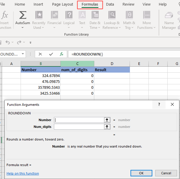
Once you open the ROUNDDOWN function, a dialog box appears as shown below.

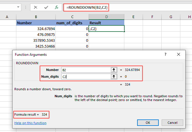
2. Enter the cell numbers in the number & num_of_digits box as shown in the image. Alternately, you can add the decimal value directly to num_digits.

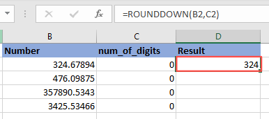
3. The resulting number in the C2 cell will be rounded to 0 decimal places.

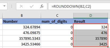
4. Use CTRL + D to copy the formula from the first cell to the last cell.

Example 2:

Rounding a number down to a positive value or dataset

Let us consider the same dataset as in example 1 and change the decimal points to numbers as shown in the image below.

Repeat the same procedure using the =ROUNDDOWN(B2,C2) formula, and you can find the decimal points rounded down to the numbers as shown.

Example 3:

Rounding a number down to a negative value or dataset

Previously, we discussed that a negative value for num_of_digits rounds down the digit to the left of decimal places.

Let us consider the following example.

Using the same formula, we can see the numbers rounded to the left of the decimal point.

We hope this article on using the ROUNDDOWN function in Excel has been helpful to you.

---